Objectives
Our two objectives of analysis were to (a) quantify the km-long length areas of interaction of subduction zone volcanism with carbonate platforms and (b) characterise the subduction volcanism as either continental or intra-oceanic depending on the proximity of the subduction zones to continent-ocean boundaries.
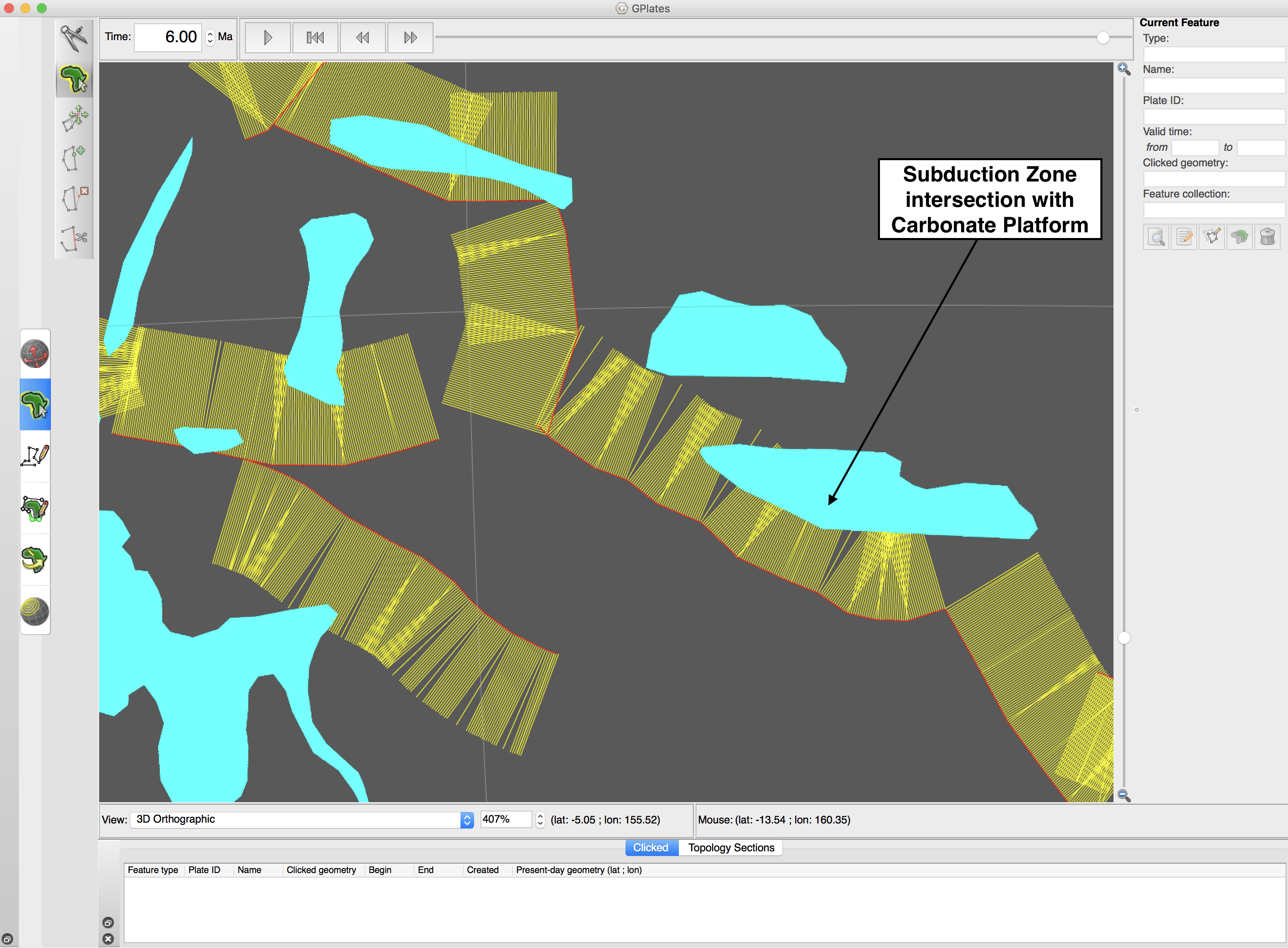
In regards to the first objective, we are interested in cases where subduction-related volcanic arcs occur within 448 km distance of a carbonate platform. We determined this inclusion radius by calculating the average distance of volcanic arc volcanoes from subduction zone trenches.
In a similar way, the second objective involved classifying volcanic arcs that occur within 448 km distance of a continent ocean boundary as continental arcs, and all others as intra-oceanic or island arcs.
Processes and Workflows
From a spatial science perspective, both objectives are somewhat similar; we are interested in the event that a polygon feature sits within a certain distance of the subducting side of a subduction zone. We designed a single workflow which was able to meet both objectives. The work flow produces subduction zone lengths at each time step which intersect a given feature (in this case, carbonate platforms or continents).
For our analysis, we used Matthews et al. (2016) plate model which gives us the plate boundary evolution from 400 Ma to present day. In addition, we used a continental terranes gpml feature file that contained continent-ocean boundary polygons which we used to reconstruct their positions at each one million year interval for the past 400 million years. In previous steps we georeferenced and assigned plate IDs to carbonate platform polygons depicting activity and accumulation over the past 400 million years.
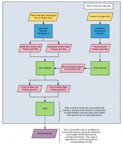
Our workflows repeats a series of operations 400 times, once for each one-million-year time step (see figure above). Our bash workflow consists of python scripts, GMT tools and AWK scriptlets organised into bash sub routine functions.
The most vital part of the workflow are the python scripts. These scripts communicate with GPlates using the pyGPlates module. Like in our subduction zone length analysis we use the script ‘resolve_topolgies_v.2.py’ to produce left and right polarity subduction zones at a given time step. We used another script ‘reconstruct_feature.py’ to reconstruct the position of our feature (continents or carbonate platforms) at a given time step.
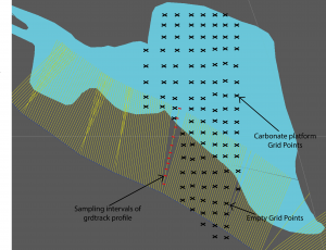
Using the reconstructed geometries of our feature, we converted them into a netCDF mask using the grdmask tool from GTM5. The netCDF grid consists of regularly spaced nodes. The interior and edges of closed polygons have a value of 1, and every other node is given a value of 0.
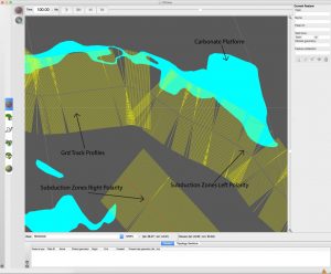
We use a GMT5 tool called grdtrack, which produces perpendicular cross profiles along a given polyline geometry – the subduction zones in our case. These cross profiles are spaced at regular distances along the subduction zone boundaries at 10 km intervals. Along each cross profile, unit intervals are specified – in our case, we used five intervals. At each interval, the mask is sampled using nearest-neighbour method and the interval node is assigned a value of either 1 or 0.
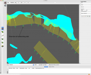
However, the cross profile extends across both sides of the subduction zone polyline. For this analysis, we are only interested in the half of the cross profile that points in the direction of subduction. Subduction zones in a previous step were classified as having either left or right polarity, and they were thus processed separately.
For the left and right polarity subduction zones, the cross profiles had to be processed separately, which is explained in this post. Using an awk script we bisected the cross profiles and removed the profile half on the not-yet-subducting side of the subduction zone. The halved cross profiles had a specified length of 448 km and they functioned as a search radius, allowing us to associate subduction zones with a particular feature if they are within 448 km of said feature.
Another awk script counted each profile that intersected with a reconstructed feature. Cross profiles with interval values of 1 are considered to be a feature intersecting profile. The profile counts of left polarity subduction zone and right polarity subduction zone were added together and multiplied by the profile spacing (10 km) to give us the total distance. The distance is appended with the corresponding time step to a dat file.
![]()
