GPlates 2.4 software and data sets

GPlates is a free desktop software for the interactive visualisation of plate-tectonics. The compilation and documentation of GPlates 2.4 data was primarily funded by AuScope National Collaborative Research Infrastructure (NCRIS).

GPlates is developed by the EarthByte Group (part of AuScope NCRIS) at the University of Sydney and the Division of Geological and Planetary Sciences (GPS) at California Institute of Technology (CalTech).

Data by the EarthByte Group is licensed under a Creative Commons Attribution 3.0 Unported License. Please cite the references listed on this page when using GPlates 2.4 data sets.

Download the latest version of GPlates here – link
View the latest GPlates user manual here – link
Download the latest GPlates tutorials here – link
Download standard file formats for GPlates here – link
Download list of plate IDs used in GPlates here – pdf

About the GPlates 2.4 GeoData

GPlates 2.4 is packaged with a range of data sets that allow users to quickly and easily get up-and-running with plate tectonic reconstructions. You can download the complete GeoData bundle as a zip file from Zenodo.

The below information details the sources of these data and relevant citations. When using GPlates and the sample data to make figures for publications, we recommend citing the original data sources as indicated below.

Features

EarthByte Global Rotation Model

The GeoData includes the Zahirovic et al. (2022) rotation file, which contains a compilation of reconstruction poles that describe the motions of the continents and oceans and applies a correction to the pre-83 Ma rotations for the Pacific plate based on Torsvik et al. (2019). These rotations are a synthesis of many previous studies; each line in the rotation file lists the original source of the corresponding poles of rotation.

The feature data provided (detailed below) are compatible with this rotation file.

Citation:

Zahirovic, S., Eleish, A., Doss, S., Pall, J., Cannon, J., Pistone, M., and Fox, P., 2022, Subduction kinematics and carbonate platform interactions: Geoscience Data Journal, doi: 10.1002/gdj3.146

Cao, X, Zahirovic, S, Li, S, Suo, Y, Wang, P, Liu, J & Muller, RD 2020, ‘A deforming plate tectonic model of the South China Block since the Jurassic’, Gondwana Research.

Müller, RD, Zahirovic, S, Williams, SE, Cannon, J, Seton, M, Bower, DJ, Tetley, MG, Heine, C, Le Breton, E, Liu, S, Russell, SHJ, Yang, T, Leonard, J & Gurnis, M 2019, ‘A global plate model including lithospheric deformation along major rifts and orogens since the Triassic’, Tectonics, vol. 38, no. Fifty Years of Plate Tectonics: Then, Now, and Beyond.

Torsvik, T.H., Steinberger, B., Shephard, G.E., Doubrovine, P.V., Gaina, C., Domeier, M., Conrad, C.P. and Sager, W.W., 2019. Pacific‐Panthalassic reconstructions: Overview, errata and the way forward. Geochemistry, Geophysics, Geosystems, DOI:10.1029/2019GC0084

Young, A, Flament, N, Maloney, K, Williams, S, Matthews, K, Zahirovic, S & Müller, RD 2018, ‘Global kinematics of tectonic plates and subduction zones since the late Paleozoic Era’, Geoscience Frontiers.

EarthByte Coastlines

The coastline for Greenland uses the Danish Geological Survey dataset, and the rest of the world uses the World Vector Shoreline from the Global Self-consistent Hierarchical High-resolution Geography (GSHHG) dataset, Version 2.3.7. The coastline data included here is a simplified version of the “high” resolution GSHHG coastline data – simplified in ArcGIS with simplification tolerance 0.05 decimal degrees (min area: 100 sq km). The coastlines are cookie-cut first using the static polygons, with a second stage applied where oceanic volcanic provinces (Johansson et al., 2018) are used to assign ages to oceanic islands related to hotspots.

For more information on GSHHG click here.

Citations:

Bohlander, J. and Scambos, T. 2007. Antarctic coastlines and grounding line derived from MODIS Mosaic of Antarctica (MOA), Boulder, Colorado USA: National Snow and Ice Data Center.

Gorny, A. J. 1977. World Data Bank II General User GuideRep. PB 271869, 10pp, Central Intelligence Agency, Washington, DC.

Johansson, L., Zahirovic, S., and Müller, R. D., 2018, The Interplay Between the Eruption and Weathering of Large Igneous Provinces and the Deep-Time Carbon Cycle: Geophysical Research Letters, v. 45, no. 11, p. 5380-5389.

Soluri, E. A., and Woodson, V. A. 1990. World Vector Shoreline, Int. Hydrograph. Rev., LXVII(1), 27-35.

Wessel, P., and Smith, W. H. F. 1996. A global, self-consistent, hierarchical, high-resolution shoreline database, J. Geophysical Res., 101(B4), 8741-8743.

EarthByte Continental Polygons

The continental polygons are a set of data containing the non-oceanic (predominantly continental) lithosphere only (consistent with the static polygons described below). These are consistent with the Zahirovic et al. (2022) model.

EarthByte Global Continent-Ocean Boundaries

The present-day Global Continent-Ocean Boundary (COB) Dataset from Müller et al. (2016) are represented as lines along passive margins and do not include active margins. The timescale used is Gee and Kent (2007). The COBs are also consistent with the Zahirovic et al. (2022) model.

Citation:

Müller, R.D., Seton, M., Zahirovic, S., Williams, S.E., Matthews, K.J., Wright, N.M., Shephard, G.E., Maloney, K.T., Barnett-Moore, N., Hosseinpour, M., Bower, D.J. & Cannon, J. 2016. Ocean Basin Evolution and Global-Scale Plate Reorganization Events Since Pangea Breakup, Annual Review of Earth and Planetary Sciences, vol. 44, pp. 107 . DOI: 10.1146/annurev-earth-060115-012211.

EarthByte Dynamic Topological Polygons

A topological network of plate polygons with “dynamic” geometries are provided for the last 410 Ma. These data are provided in gpml (GPlates native) format and so require GPlates to be effectively visualised. Further information of this collection of data can be found here. The dynamic “continuously-closing” topological polygons are consistent with the Zahirovic et al. (2022) model.

Citation:

Cao, X, Zahirovic, S, Li, S, Suo, Y, Wang, P, Liu, J & Muller, RD 2020, ‘A deforming plate tectonic model of the South China Block since the Jurassic’, Gondwana Research.

EarthByte Flowlines

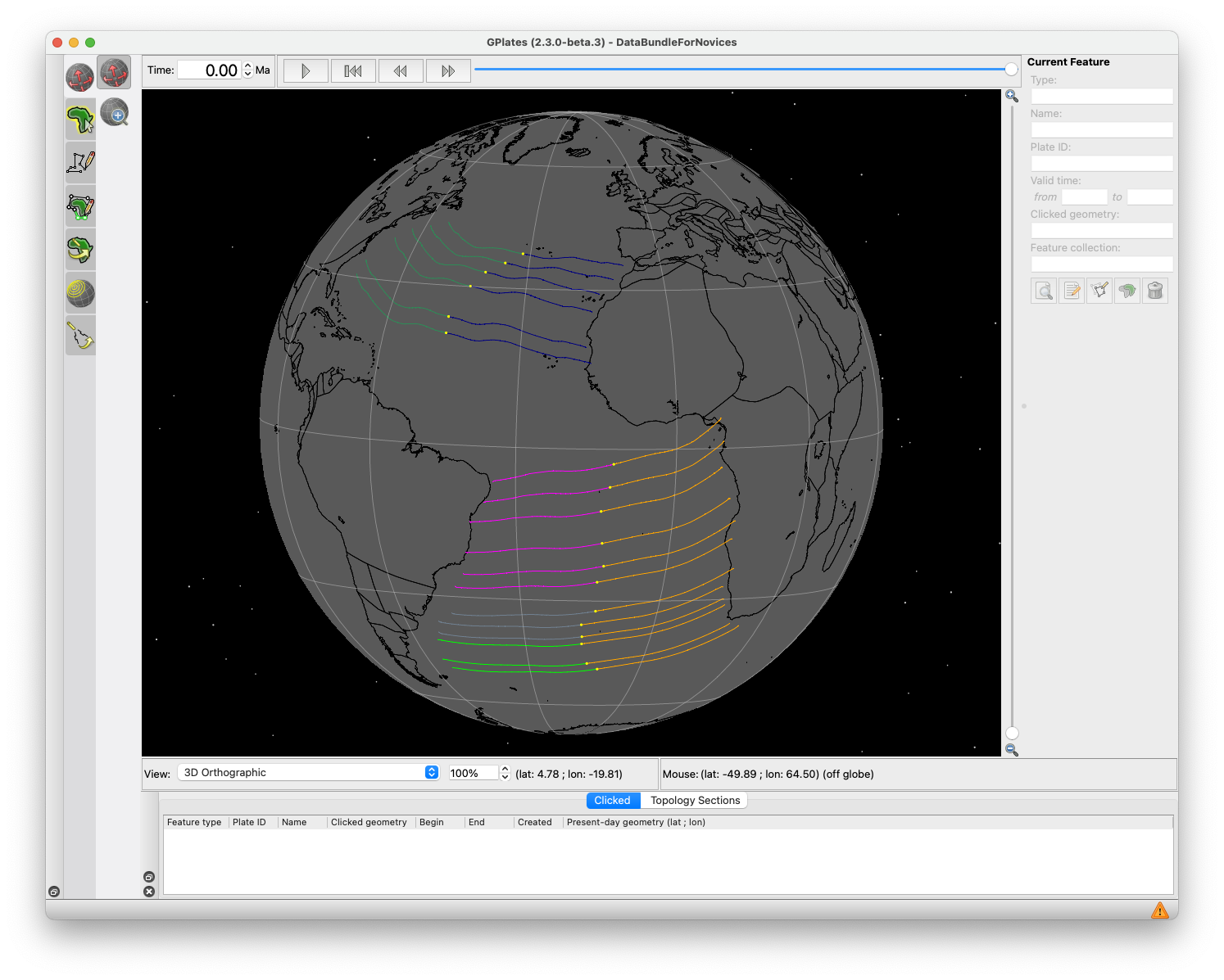
This directory contains examples of plate motion “flowlines” across the Atlantic Ocean that have been generated in GPlates. The directory contains a .gpml file which contains seed points at several locations along the Mid-Atlantic Ridge. When loaded with a rotation file the flowlines will be drawn to reflect the relative motion between the plate pair either side of the mid-ocean ridge.

The flowlines will be reconstructed according to the rotation file that is loaded when they are opened but were created using a ridge axis location that is consistent with the Zahirovic et al. (2022) model.

EarthByte Grid Marks

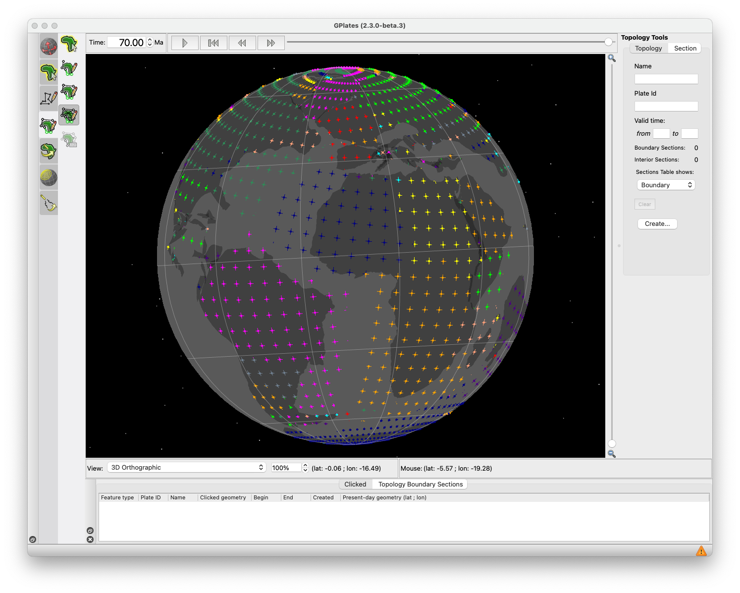
The grid marks included in the Sample Data have been cookie-cut using the Zahirovic et al. (2022) model.

EarthByte Hotspots

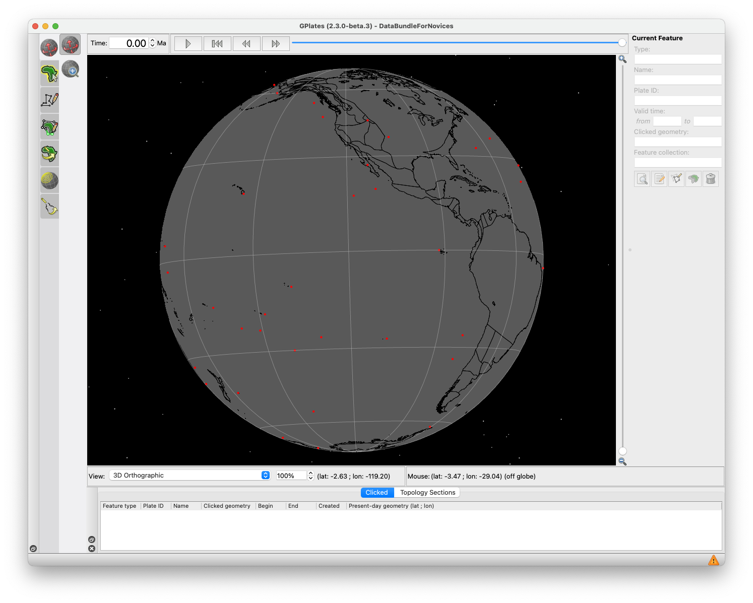
The hotspot/plume locations are a compilation of present day surface hotspot/plume locations from Whittaker et al. (2015), and are represented as points and are split in Pacific and Indo/Atlantic domains. Locations were compiled from Montelli et al. (2004), Courtillot et al. (2003), Steinberger et al. (2000) and Anderson and Schramm (2005). Plumes closer than 500 km were combined into an averaged location.

Citation:

Whittaker, J., Afonso, J., Masterton, S., Müller, R., Wessel, P., Williams, S., and Seton, M., 2015, Long-term interaction between mid-ocean ridges and mantle plumes: Nature Geoscience, v. 8, no. 6, p. 479-483, doi: 10.1038/ngeo2437.

EarthByte Isochron File

This directory contains the Seton et al. (2020) Ocean Floor Isochron Dataset. The isochrons are represented as lines and do not include reconstructed isochrons. The timescale used is Gee and Kent (2007). They are consistent with the Zahirovic et al. (2022) model.

Citation:

Gee, J. S., and Kent, D. V., 2007, Source of oceanic magnetic anomalies and the geomagnetic polarity time scale: Treatise on Geophysics, vol. 5: Geomagnetism, p. 455-507.

Seton, M., Müller, R. D., Zahirovic, S., Williams, S., Wright, N. M., Cannon, J., Whittaker, J. M., Matthews, K. J., and McGirr, R., 2020, A Global Data Set of Present-Day Oceanic Crustal Age and Seafloor Spreading Parameters: Geochemistry, Geophysics, Geosystems, v. 21, no. 10.

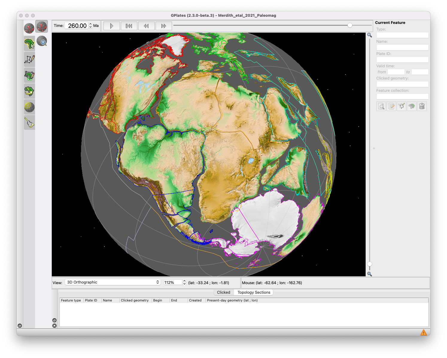
EarthByte Paleomagnetic Data

The paleomagnetism data sets are from the Global Paleomagnetic Database (GPMDB; https://gpmdb.net/). The data are provided in GPML format.

Citation:

Pisarevsky, S. A., Li, Z. X., Tetley, M. G., Liu, Y., & Beardmore, J. P. (2022). An updated internet-based Global Paleomagnetic Database. Earth-Science Reviews, 104258, doi:10.1016/j.earscirev.2022.104258

EarthByte Seafloor Fabric

The ‘SeafloorFabric’ folder within the sample data contains a set of geometries that define the tectonic fabric of the world’s oceans. The data are taken from a global community data set of fracture zones (FZs), discordant zones, propagating ridges, V-shaped structures and extinct ridges, digitized from vertical gravity gradient (VGG) maps. More information on the tectonic fabric of the ocean basins can be found here.

Citation:
Matthews, K. J., Müller, R. D., Wessel, P., Whittaker, J. M. 2011. The tectonic fabric of the ocean basins, The Journal of Geophysical Research. Doi: 10.1029/2011JB008413.

EarthByte Global Spreading Ridge File

The Zahirovic et al. (2022) model spreading ridge dataset includes present day spreading ridges and extinct ridges, which are represented as lines. The timescale used is Gee and Kent (2007).

Citation:

Zahirovic, S., Eleish, A., Doss, S., Pall, J., Cannon, J., Pistone, M., and Fox, P., 2022, Subduction kinematics and carbonate platform interactions: Geoscience Data Journal, doi: 10.1002/gdj3.146

EarthByte Static Polygons

Static polygons allow plate IDs to be assigned to other sets of data and to reconstruct raster data. These polygons, and the set of isochrons defining the age of the ocean floor.

Citation:

Zahirovic, S., Eleish, A., Doss, S., Pall, J., Cannon, J., Pistone, M., and Fox, P., 2022, Subduction kinematics and carbonate platform interactions: Geoscience Data Journal, doi: 10.1002/gdj3.146

Müller, R. D., Zahirovic, S., Williams, S. E., Cannon, J., Seton, M., Bower, D. J., Tetley, M. G., Heine, C., Le Breton, E., Liu, S., Russell, S. H. J., Yang, T., Leonard, J., and Gurnis, M., 2019, A global plate model including lithospheric deformation along major rifts and orogens since the Triassic: Tectonics, v. 38, no. Fifty Years of Plate Tectonics: Then, Now, and Beyond.

EarthByte Large Igneous Provinces and Volcanic Provinces

Large Igneous Provinces represent the world’s major voluminous plume-related volcanic products.

Citation:

Volcanic Provinces represent a combination of Large Igneous Provinces, age-progressive plume volcanic products and other volcanic features.

Citation:

Johansson, L., Zahirovic, S., and Müller, R. D., 2018, The interplay between the eruption and weathering of Large Igneous Provinces and the deep-time carbon cycle: Geophysical Research Letters, doi:10.1029/2017GL076691.

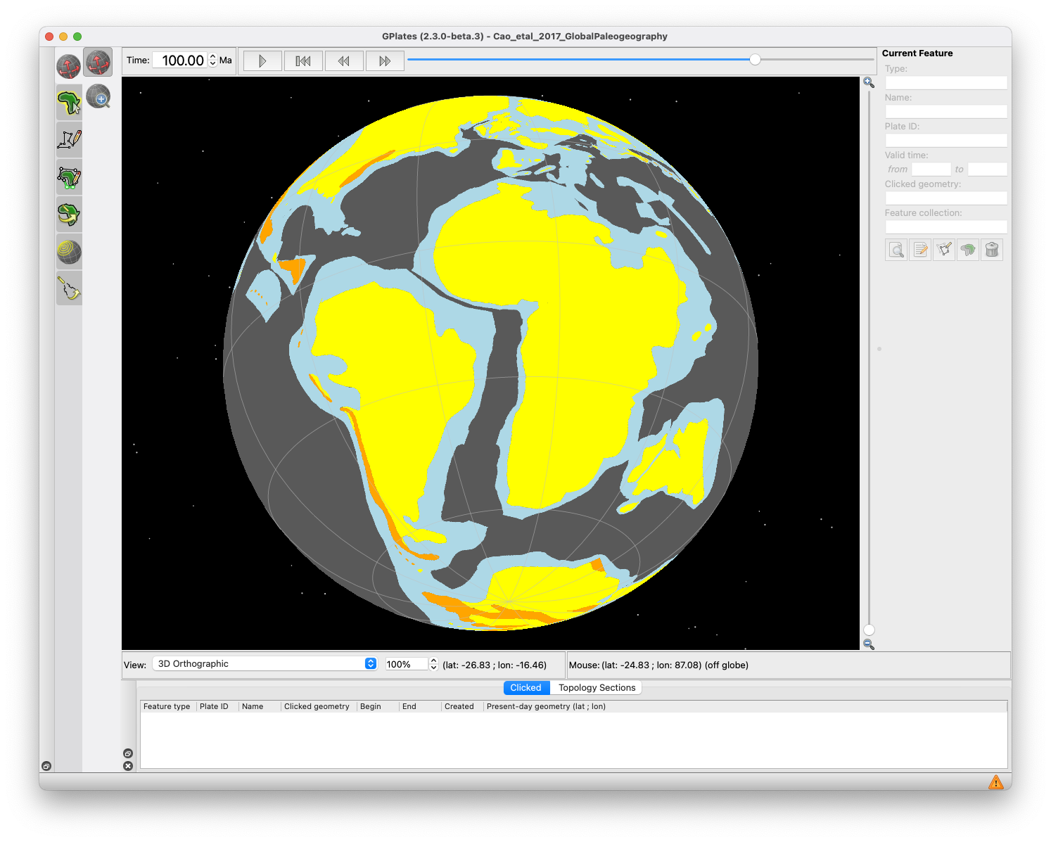
EarthByte Paleogeography

Global paleogeography from the Devonian to present is composed of a series of polygon layers that represent shallow marine, mountaineous, icesheet, and emergent land.

Citation:

Cao, W., Zahirovic, S., Flament, N., Williams, S., Golonka, J., and Müller, R. D., 2017, Improving global paleogeography since the late Paleozoic using paleobiology: Biogeosciences, v. 14, no. 23, p. 5425-5439, DOI:10.5194/bg-14-5425-2017.

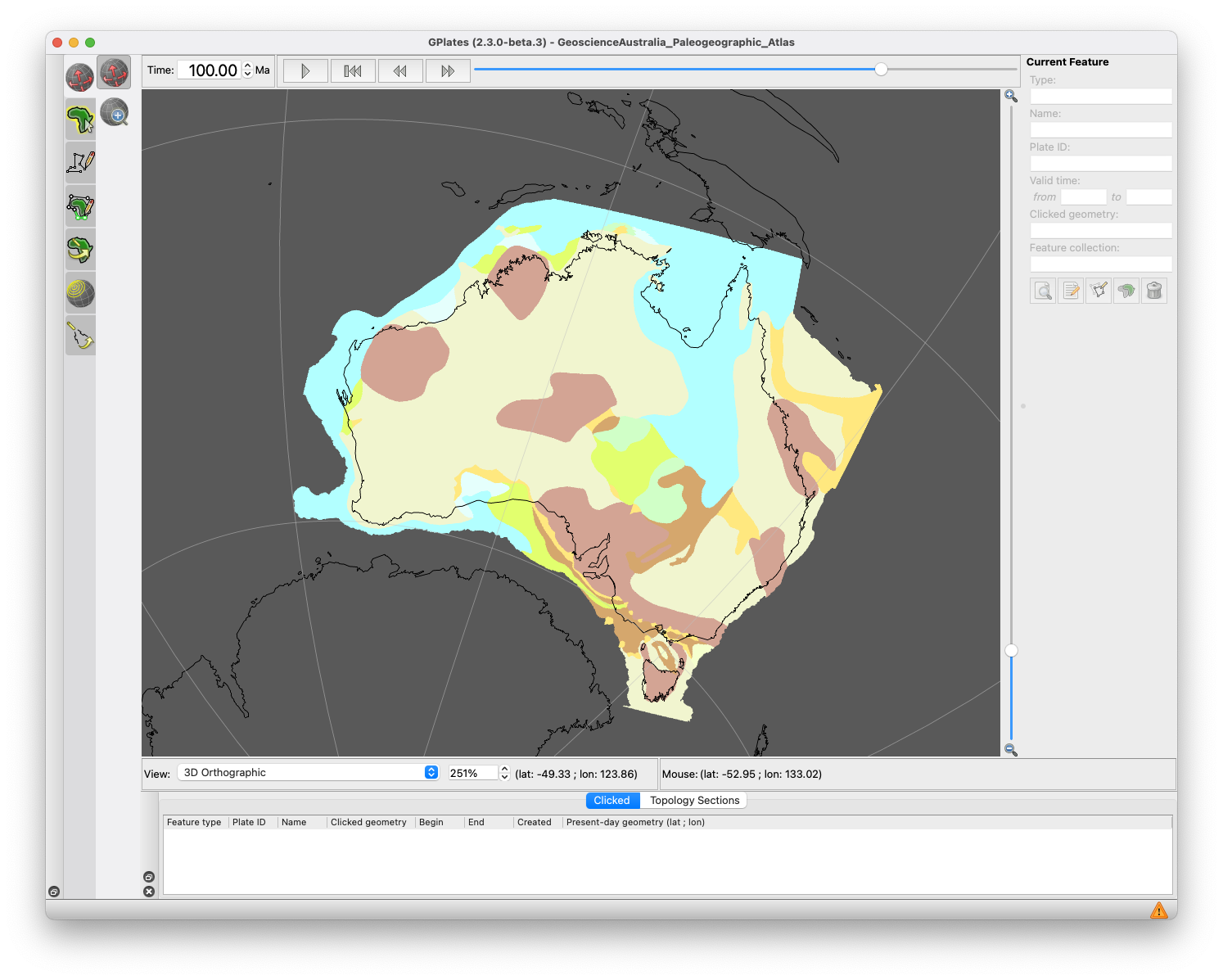
Regional paleogeography of Australia for the Phanerozoic is adapted from the Australian Paleogeographic Atlas, and represents a range of paleo-environments.

Citation:

Totterdell, J.M., Cook, P.J., Bradshaw, M.T., Wilford, G.E., Yeates, A.N., Yeung, M., Truswell, E.M., Brakel, A.T., Isem, A.R., Olissoff, S., Strusz, D.L., Langford, R.P., Walley, A.M., Mulholland, S.M., Beynon, R.M., 2001, Palaeogeographic Atlas of Australia: Geoscience Australia.

EarthByte Alternative Plate Reconstructions

This is the rigid model presented in Muller et al. (2022), which is a variant of the Merdtih et al. (2021) model. It includes the original paleomagnetic reference frame, as well as two mantle reference frames, including an optimised mantle reference frame and a no-net-rotation reference frame.

Citation:

Müller, R. D., Cannon, J., Tetley, M., Williams, S. E., Cao, X., Flament, N., Bodur, Ö. F., Zahirovic, S., and Merdith, A., 2022, A tectonic-rules based mantle reference frame since 1 billion years ago–implications for supercontinent cycles and plate-mantle system evolution: Solid Earth, p. 1-42, doi: 10.5194/se-13-1127-2022

Merdith, A., Williams, S. E., Collins, A. S., Tetley, M. G., Mulder, J. A., Blades, M. L., Young, A., Armistead, S., Cannon, J., Zahirovic, S., and Müller, R. D., 2021, Extending Whole-Plate Tectonic Models into Deep Time: Linking the Neoproterozoic and the Phanerozoic: Earth Science Reviews, v. 214.

Rasters

Note: The resolution of the provided rasters has been limited to reduce the file size of the GPlates package. The original data sets are available in higher resolutions from links provided but we also provide a .nc file for convenience.

Each raster has at least three associated files, a netcdf grid, a .jpg/.png/.tif image file AND also a GPlates .gpml file. For easiest results, open the .gpml file in GPlates. GPlates will then generate some cache files that help it display the raster. Generating the cache files takes up some hard drive space and can take a minute to generate them the first time the rasters are loaded. Each subsequent loading of the raster using the .gpml file will be quicker, as GPlates will use the already-generated cache files. The Seafloor_Age_Grid contains a third .gproj file which is the best one to load this raster. Also contained in each of these folders is a Legend image which gives an indication what the colours refer to.

The quickest way to load these rasters in GPlates is to use the File > Open Feature Collection and point to the .gpml file on your machine. Alternatively, you can also click and drag the .gpml file onto the globe in the GPlates main window. The general approach to loading your own rasters in GPlates is to do the following:

1. Open GPlates
2. Pull down the GPlates File menu, select Import and then select Import Raster
3. Navigate to and click on the appropriate file
4. Leave the default to be “band_1” and click Continue
5. Specify the geographic extent (unless it is a NETCDF numerical grid where that information is automatically detected) and click Continue
6. Click Done to create a new feature collection, and GPlates will create a .gpml file following the name of the raster

Note: When importing your own raster, GPlates will automatically generate a GPML file. To save time, next time you can just load the GPML file, and thus skip the import raster step. When loading rasters for the first time, GPlates may take a few minutes to generate the cache files that will enable efficient viewing. These only need to be generated once, however, if they are deleted, they will be re-generated.

In order to reconstruct these features, you will need to load in the underlying rotation model (.rot file) cookie-cut the data using the Static Polygon files, which can be downloaded above.

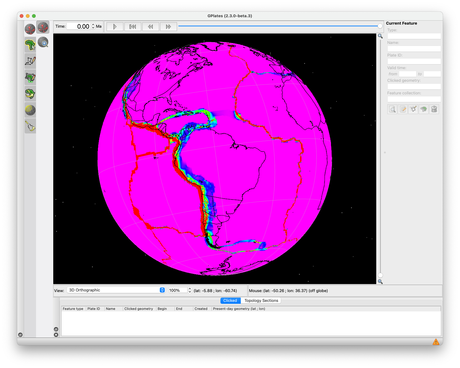
Global Present Day Age Grid

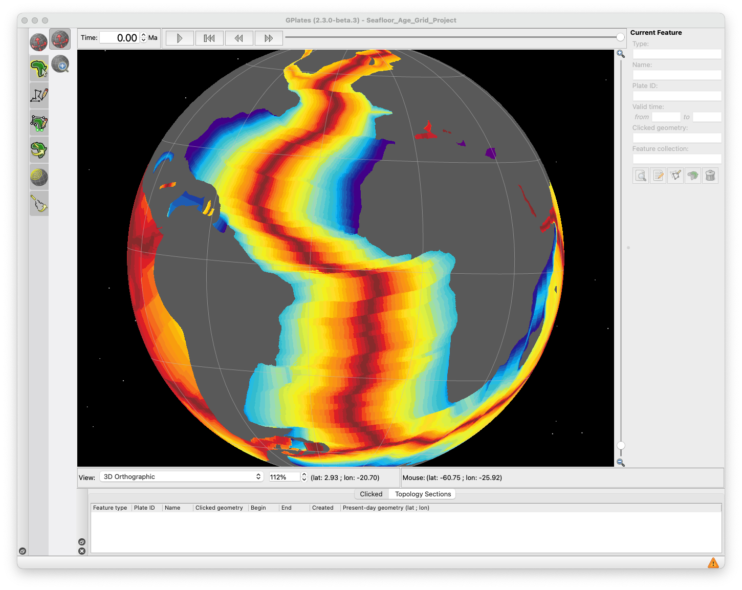
NetCDF numerical grid of seafloor age consistent with the Muller et al. (2016) produced by the EarthByte group with 6 arc minute resolution. It is best to open the Project (.gproj), as this will import the correct colour palette settings. As this is a grid file (.nc) no legend is required, however, this is accessible from the GPlates Layers dialog. A higher-resolution 2 arc minute grid is available from here.

Citation:

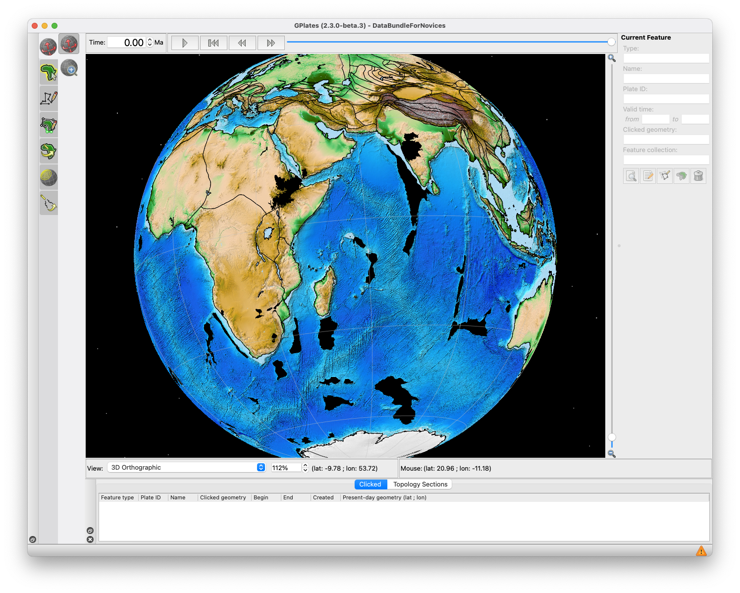
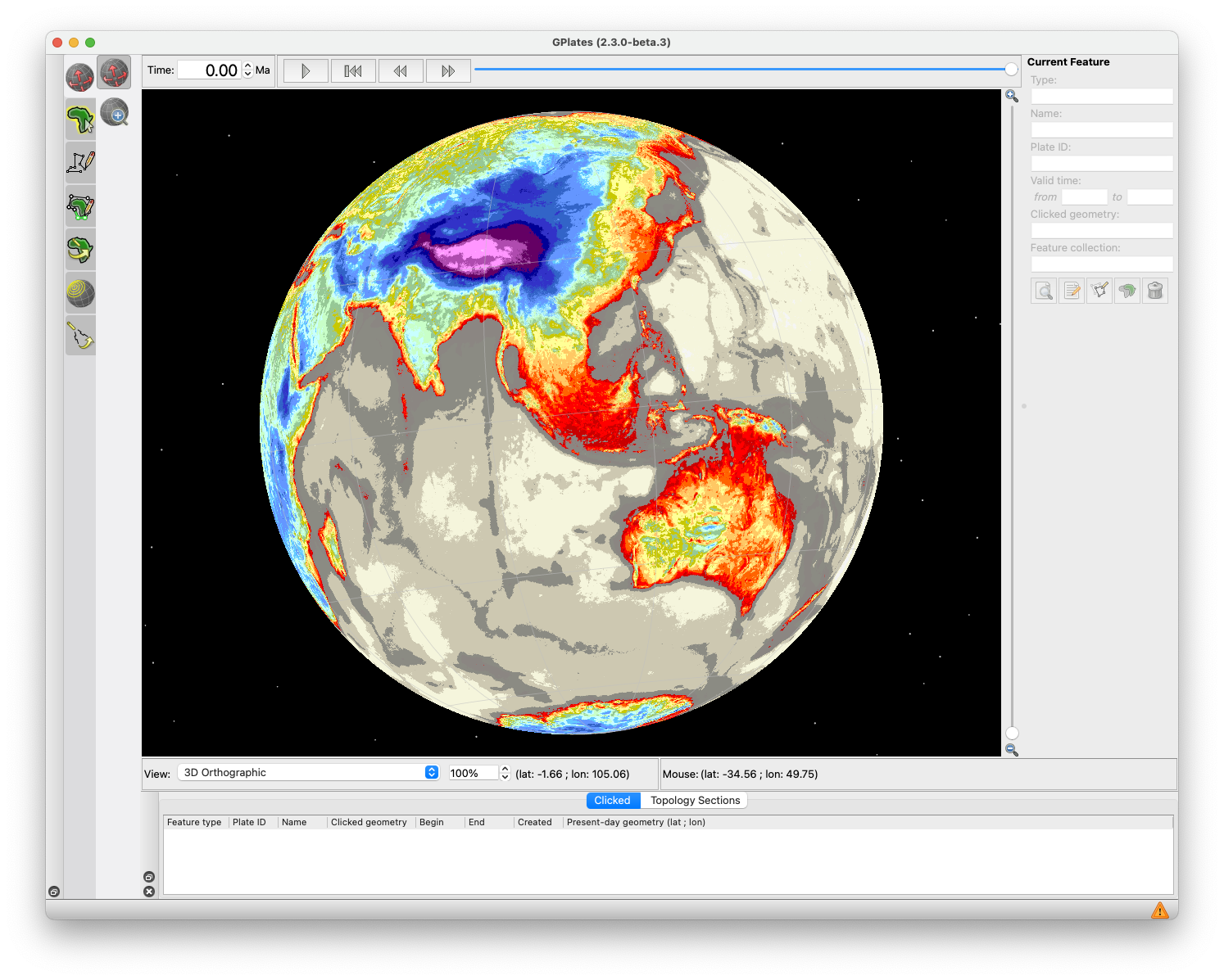
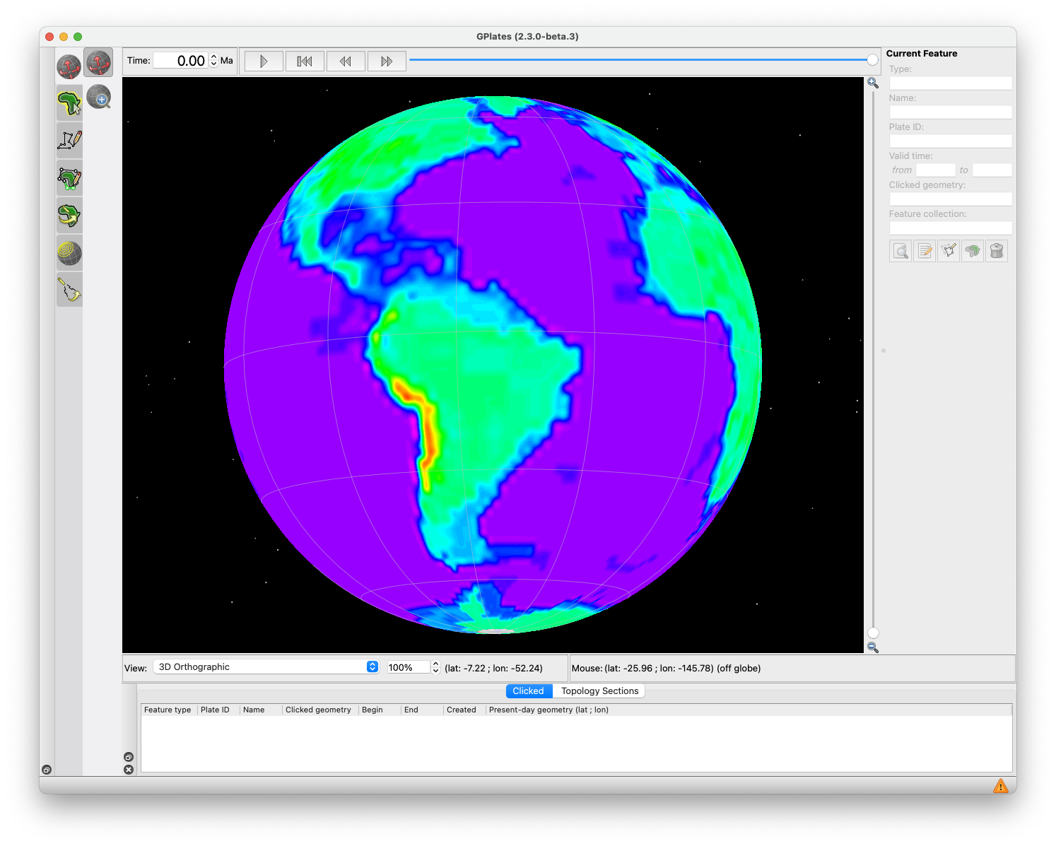
Global Topography

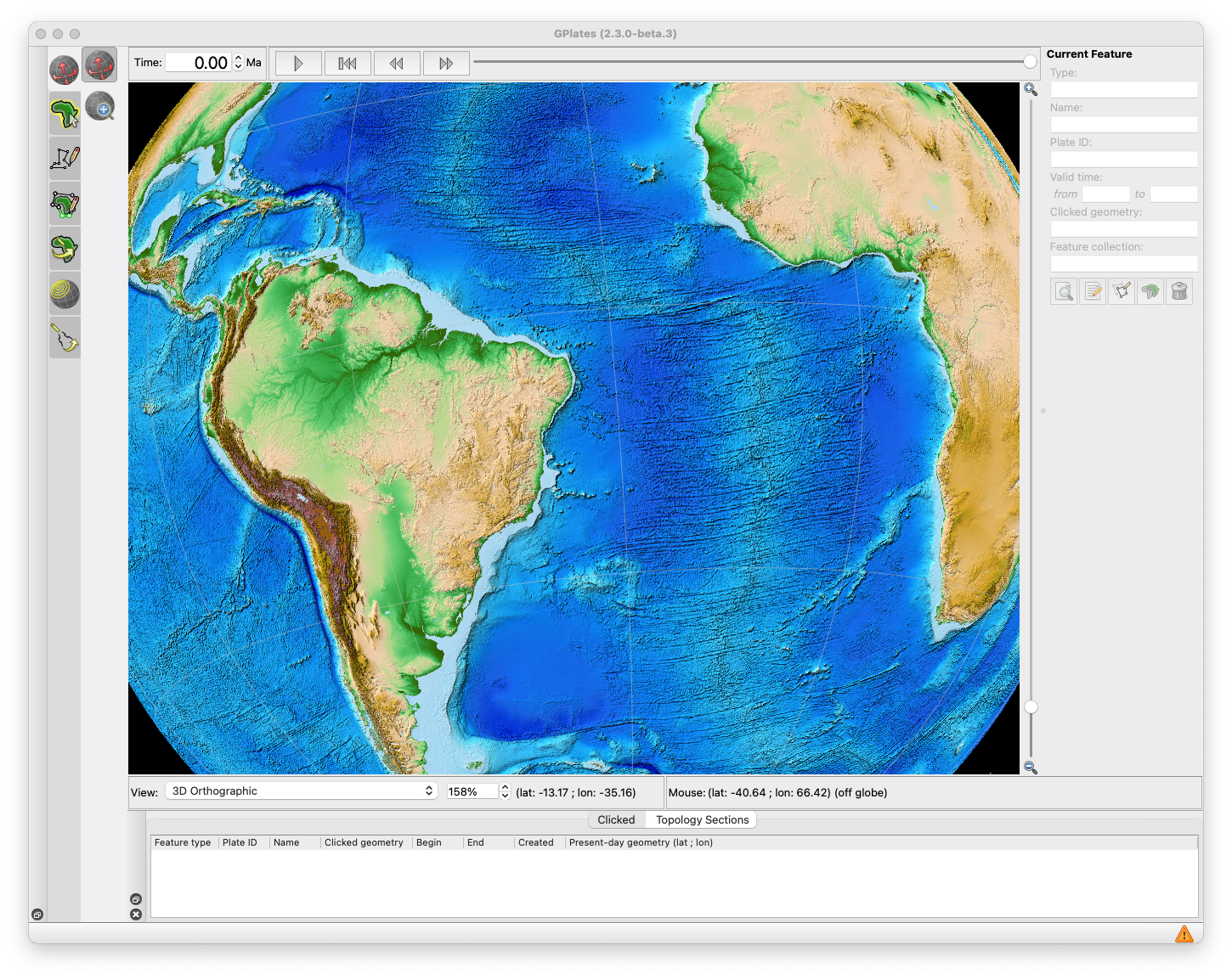
Colour grid of present-day 1 arc minute resolution topography (ETOPO1) from Amante et al. (2009), with white regions representing ice sheets. This is available from the National Geophysical Data Center (NGDC). More information, and the original data in a variety of grid formats, can be found here.

Citation:
Amante, C. and Eakins, B. W. 2009. ETOPO1 1 Arc-Minute Global Relief Model: Procedures, Data Sources and Analysis. NOAA Technical Memorandum NESDIS NGDC-24, 19.

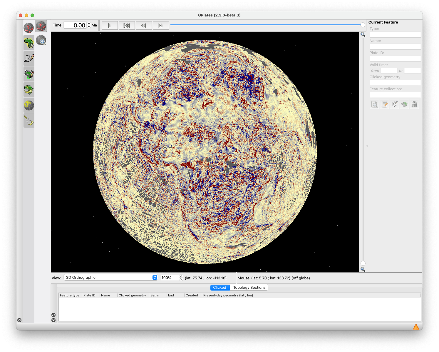
Global Free Air Gravity Anomalies

The image of free air gravity is generated from Sandwell et al. (2014) and from the Danish National Space Centre (DNSC). In ploar regions, north of 80N and south of 80S the gravity anomalies are from the DNSC08. For latitudes within +/- 80 degrees, the gravity model of Sandwell et al. (2014) is used and this is the .nc file that is provided. More information, as well as the original data sets in their full resolution, can be found here for the DNSC and here for Sandwell et al. (2014).

Citations:

Sandwell, D. T., Müller, R. D., Smith, W. H. F., Gracia, E. and Francis, E. 2014. New global marine gravity field model from CryoSat-2 and Jason-1 reveals buried tectonic structure. Science, Vol. 346 (6205), pp. 65-67. Doi: 10.1126/science.1258213.

Andersen, O. B., Knudsen, P. and Berry, P. 2010. The DNSC08GRA global marine gravity field from double retracked satellite altimetry, Journal of Geodesy, Volume 84, Number 3. DOI: 10.1007/s00190-009-0355-9.

Andersen, O. B., 2010. The DTU10 Gravity field and Mean sea surface. Second international symposium of the gravity field of the Earth (IGFS2), Fairbanks, Alaska.

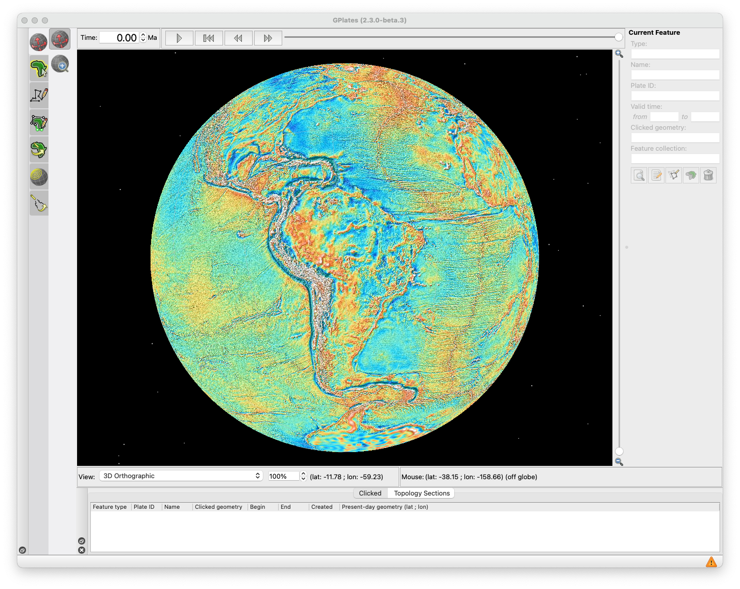
Vertical Gravity Gradient (VGG)

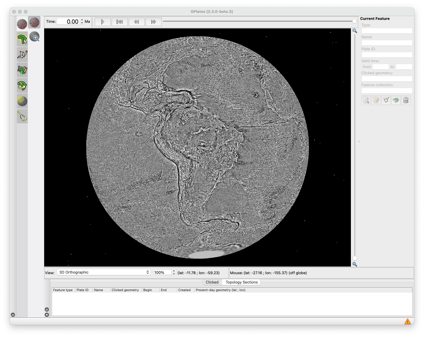
The Vertical Gravity Gradient (VGG) grid is from Sandwell et al. (2014). More information, as well as the original data sets in their full resolution, can be found here for the DNSC and here for Sandwell et al. (2014).

Citations:

Sandwell, D. T., Müller, R. D., Smith, W. H. F., Gracia, E. and Francis, E. 2014. New global marine gravity field model from CryoSat-2 and Jason-1 reveals buried tectonic structure. Science, Vol. 346 (6205), pp. 65-67. Doi: 10.1126/science.1258213.

Bouguer Gravity Anomalies

Bouguer gravity anomalies from the World Gravity Map (Balmino et al., 2012).

Citations:

Balmino, G., Vales, N., Bonvalot, S. and Briais, A., 2012. Spherical harmonic modeling to ultra-high degree of Bouguer and isostatic anomalies. Journal of Geodesy. July 2012, Volume 86, Issue 7, pp 499-520 , DOI 10.1007/s00190-011-0533-4.

Isostatic Gravity Anomalies

Isostatic gravity anomalies from the World Gravity Map (Balmino et al., 2012).

Citations:

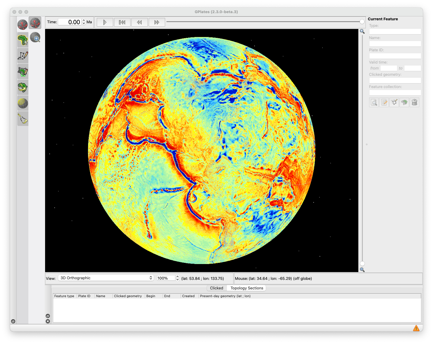
Global Magnetic Anomalies (EMAG2)

Colour grid of magnetic anomalies from EMAG2 (Maus et al., 2009). This raster does not use the directional gridding to fill gaps, and so better represents the raw magnetic data. More information, and the original data at full resolution, can be found here.

Citation:

Maus, S., Barckhausen, U., Berkenbosch, H., Bournas, N., Brozena, J., Childers, V., Dostaler, F., Fairhead, J., Finn, C., and von Frese, R., 2009, EMAG2: A 2-arc min resolution Earth Magnetic Anomaly Grid compiled from satellite, airborne, and marine magnetic measurements: Geochemistry, Geophysics, Geosystems, v. 10, no. 8, p. Q08005, doi:10.1029/2009GC002471.

Global Geology

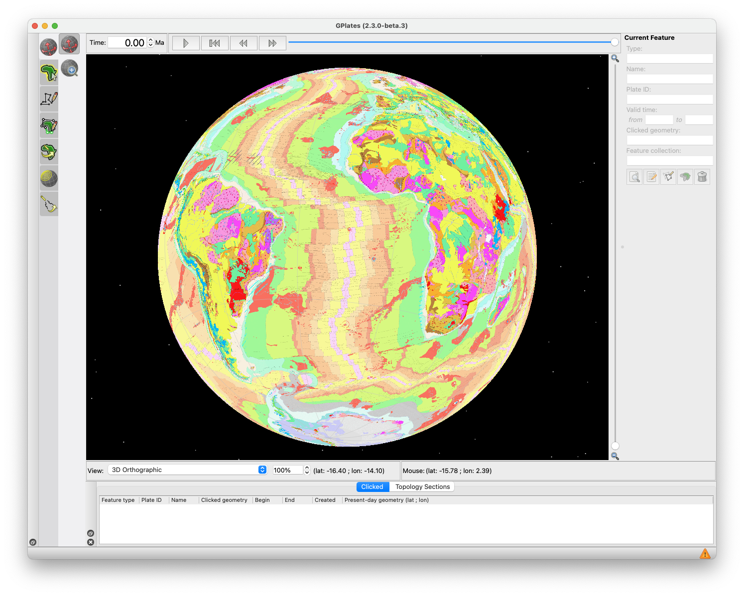
World geological map from Bouysse (2014) published by the UNESCO CGMW program.

Citation:

Bouysse, P., 2014, Geological Map of the World at 1:35 000 000.

Crustal Thickness

Crustal thickness model (CRUST 2.0) from Laske et al. (2000).

Citation:

Laske, G., Masters, G., and Reif, C., 2000, CRUST 2.0: A new global crustal model at 2×2 degrees, Institute of Geophysics and Planetary Physics, The University of California, San Diego, website: http://igppweb.ucsd.edu/~gabi/crust2.html.

Crustal Strain

Second invariant of strain rate from Kreemer et al. (2014).

Citation:

Kreemer, C., Blewitt, G., and Klein, E. C., 2014, A geodetic plate motion and global strain rate model: Geochemistry, Geophysics, Geosystems, v. 15.

Time-dependent Raster

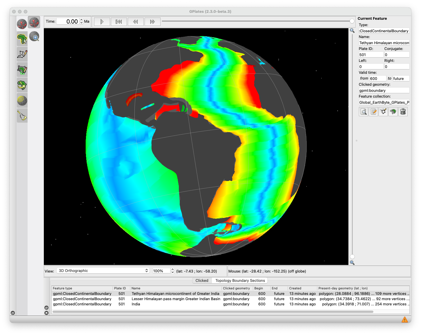
Global Age-coded Slabs in P-wave Tomography

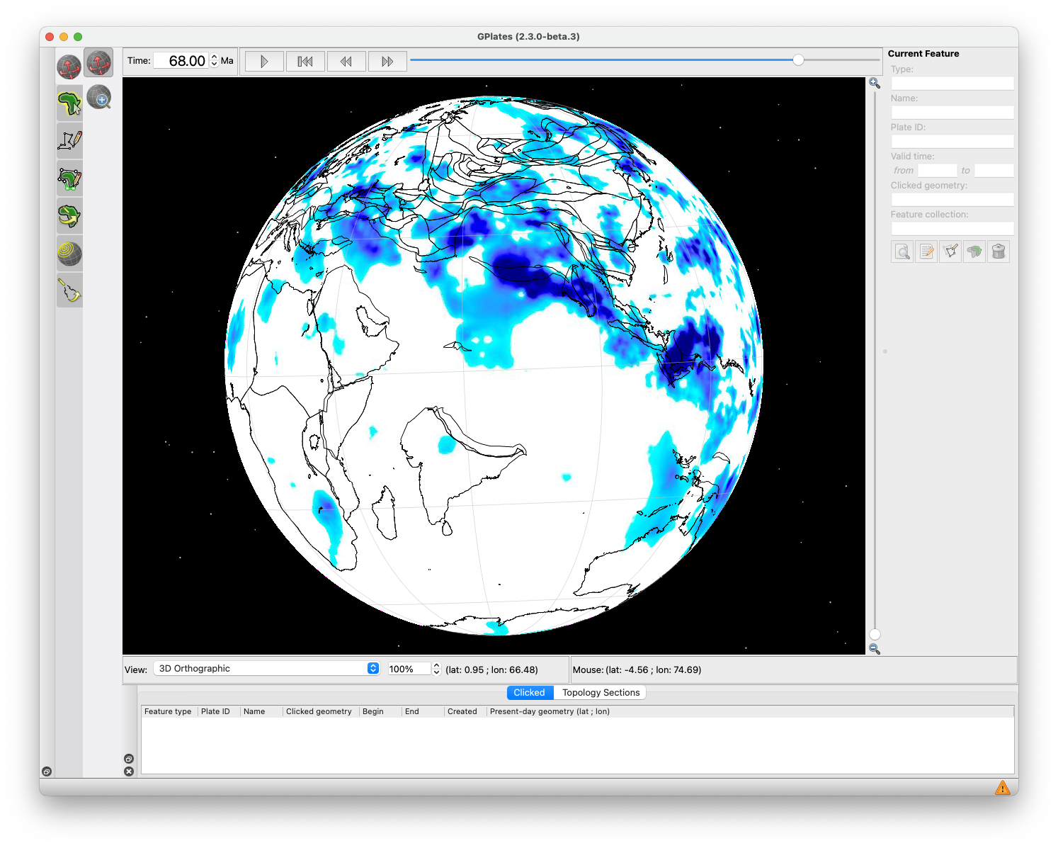
GPlates also has the ability to display time-dependent rasters. These rasters can e global or regional, and the suffix to the filename is a dash or underscore followed by an integer age in millions of years before present. In the Sample Data we include a time-dependent raster of slabs age-coded from the MIT-P P-wave seismic tomography (Li et al., 2008), where slabs are assumed (on the first order) to sink vertically with a constant sinking rate. The sinking rate applied here is 3 cm/yr in the upper mantle, and 1.2 cm/yr in the lower mantle. The quickest way to visualise this dataset in GPlates is to load the. gpml file (MIT-P08-Asia-UM30 LM12.gpml) as described above.However, the first time the time-dependent rasters are loaded, GPlates will need to generate cache files for eachdepth/time layer. This process will take some minutes, and will take up a total of about 350 Mb of hard disk space. GPlates requires that the rasters follow the same file naming format, and that they are all exactly the same dimensions (pixel width and height).

Citation:

Li, C., van der Hilst, R., Engdahl, E. and Burdick, S., 2008. A new global model for P wave speed variations in Earth’s mantle. Geochemistry, Geophysics, Geosystems, 9(5): 21, doi: 10.1029/2007GC001806.

Global Time-evolving Seafloor Age Grid

NetCDF numerical grid of seafloor age consistent with the Zahirovic et al. (2022) model with 6 arc minute resolution. It is best to open the Project (.gproj), as this will import the correct colour palette settings. As this is a grid file (.nc) no legend is required, however, this is accessible from the GPlates Layers dialog.

Citation:

Zahirovic, S., Eleish, A., Doss, S., Pall, J., Cannon, J., Pistone, M., and Fox, P., 2022, Subduction kinematics and carbonate platform interactions: Geoscience Data Journal, doi: 10.1002/gdj3.146

Download time-evolving seafloor age-grid

The general approach to loading your own time-dependent rasters in GPlates is to do the following:

1. Open GPlates
2. Pull down the GPlates File menu, select Import and then select Import Time-Dependent Raster
3. You can select an entire folder by clicking the “Add directory” button, or add files by clicking the “Add files” button
4. GPlates will take some time to generate the cache files, after which you need to click Continue
5. Leave the default to be “band_1” and click Continue
7. Specify the geographic extent (unless it is a NETCDF numerical grid where that information is automatically detected) and click Continue
8. Click Done to create a new feature collection, and GPlates will create a .gpml file following the name of the time-dependent raster

Note: You will only need to load the GPML the next time you need to use the time-dependent raster, which allows you to bypass the re-import process.

Any questions, please email:

Dietmar Muller: dietmar.muller@sydney.edu.au

Sabin Zahirovic: sabin.zahirovic@sydney.edu.au

Maria Seton: maria.seton@sydney.edu.au